Unified Generative-Predictive Modeling for 4D Scene Understanding

A single diffusion transformer treats RGB video, depth, and camera rays as symmetric modalities, casting visual generation and geometric prediction as the same conditional-completion problem. The result is one model that does camera-controlled video synthesis, depth, and pose, and improves itself by drawing more samples at inference time.

1 · Why unify generation and prediction?

A photo or a short video shows only one slice of a scene: visible surfaces from one viewpoint at one moment in time. Robust 4D understanding has to recover the things the camera did not capture: the unobserved side of an object, the camera’s pose, the metric depth at every pixel, and how those quantities evolve through time. The field has historically split this job in two.

Feedforward predictors regress geometry directly from pixels, often with strong supervision and large datasets . They are fast and accurate inside their training distribution, but they collapse to a single deterministic answer and degrade when the observations are sparse, ambiguous, or out of distribution.

Generative video models learn rich appearance priors and can hallucinate plausible completions, but they have no native notion of metric depth or 3D structure; their outputs can look right while being geometrically inconsistent .

Chaining the two pipeline-style works only when one stage is willing to treat the other’s output as ground truth, which rarely holds.

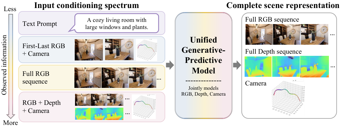
Scientific question. Can a single model do both, by treating generation and prediction as different conditional queries on the same joint distribution over appearance and geometry, and does that unification produce real, measurable benefits (heterogeneous training, posterior search, robustness to sparse observations)?

RGB, depth, and camera pose are complementary observations of a dynamic scene: RGB describes appearance, depth describes visible 3D structure, and camera pose describes viewpoint. Depending on what is observed, the missing components may be future RGB frames, dense depth, or camera geometry. We answer the question above with a unified generative-predictive model that represents RGB, depth, and camera rays as spatially aligned tokens in a shared multimodal transformer and trains it via diffusion forcing . The clean/noisy pattern across modality-frame groups specifies the task. The same weights then perform camera-controlled video generation, dense video depth estimation, and camera pose recovery, and crucially, the generative formulation lets us sample multiple 4D scene hypotheses at inference time and pick the one with the lowest cross-modal reprojection error.

One model, three modalities, many tasks. — **Figure 1 · Unified conditional completion.** Given any partial observation, such as a text prompt, a single RGB image, an RGB sequence, camera poses (rays), or depth, the same model fills in the rest. Camera-controlled generation, depth estimation, and pose recovery are different masks on the same denoiser.

2 · Background and prior work

Geometric prediction. Feedforward 3D / 4D regressors (DUSt3R , VGGT , $\pi^3$ ) map pixels to depth, point maps, or pose in one pass. Recent diffusion-based methods adapt generative priors for specific geometric outputs: RayDiffusion for camera rays, Marigold , DepthCrafter , and ChronoDepth for depth, and Geo4D for joint 4D reconstruction. Each is still a unidirectional RGB → geometry map trained on strictly paired data.

Geometry-aware video generation. Video world models have moved from pure pixel synthesis toward injecting 3D structure for spatial consistency or accepting camera trajectories as control . The closest concurrent work (One4D and WorldReel ) jointly emits RGB plus 4D geometric quantities, but along fixed input/output paths.

The gap we close. All of the above either (i) treat geometry as a byproduct of generation, or (ii) treat generation as one-way prediction. None of them treats RGB, depth, and camera geometry as symmetric modalities in a single any-to-any conditional distribution. Doing so requires (a) modality-symmetric tokenization, (b) a training objective that handles heterogeneous, partially annotated data, and (c) an inference procedure that exploits the joint distribution. The Mixture-of-Transformers backbone plus diffusion forcing are the right tools, and that is what we use.

Philosophically the formulation echoes perception as inference from cognitive science : scene understanding is generating-and-checking, not one-pass regression.

3 · Method

3.1 A shared 4D scene representation

A 4D scene is a sequence of $N=50$ frames; each frame $i$ has an RGB image $I_i$, a depth map $D_i$, and camera parameters $C_i = (K_i, T_i)$.

To put camera geometry in the same spatial container as RGB and depth we convert $C_i$ into a dense Plücker ray map :

\[R_i(u,v) = \big(\,\mathbf{d}_i(u,v),\ \mathbf{m}_i(u,v)\,\big), \qquad \mathbf{m}_i(u,v) = \mathbf{o}_i \times \mathbf{d}_i(u,v),\]

where $\mathbf{o}_i$ is the camera center and $\mathbf{d}_i(u,v)$ the unit viewing direction in world coordinates. Ray direction carries orientation + intrinsics; ray moment carries the camera center up to a global scene scale. Unlike raw extrinsics or token-form camera embeddings, the per-pixel ray map places camera geometry on the same $(u,v,i)$ grid as RGB and depth, so cross-modal attention and reprojection are well-defined. Depth is reparameterized to a bounded disparity-like channel

\[\tilde{D} = \frac{2}{1 + D/s} - 1 \in [-1, 1],\]

with a single clip-level scale $s$ that is also applied to the ray moments. This shared normalization is what makes cross-modal constraints like photometric reprojection numerically well defined.

The full scene is then ${(I_i, D_i, R_i)}_{i=1}^{N}$: three image-shaped streams over the same $(u,v,i)$ grid.

3.2 Mixture-of-Transformers backbone

Generative-predictive transformer architecture. — **Figure 2 · Architecture.** RGB and depth are encoded by a frozen Wan2.1 VAE; ray maps are packed directly into latents at the VAE resolution. Modality-specific patch embeddings and feed-forward layers preserve per-modality statistics, while a *shared multimodal self-attention* mixes information across appearance, depth, and rays. Per-token diffusion timesteps drive adaptive modulation.

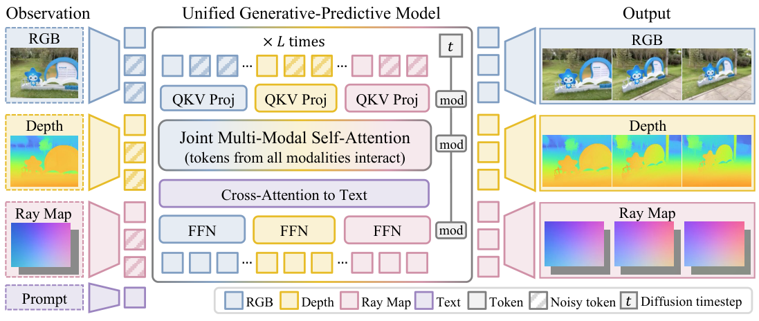
We initialize from Wan2.1-T2V-1.3B (a 1.3B-parameter video DiT) and extend it into a four-stream Mixture-of-Transformers :

\[z = [\,z^I;\ z^D;\ z^{R_d};\ z^{R_m}\,],\]

with separate streams for RGB, depth, ray direction, and ray moment. Each clip is 50 frames at $240\times320$; after VAE encoding (stride $4\times8\times8$) each modality becomes a $14 \times 30 \times 40$ latent with 16 channels. A 3D patch size of $[1,2,2]$ yields $4{,}200$ tokens per modality and $16{,}800$ tokens per clip. Ray maps bypass the VAE; four consecutive 3-channel ray frames pack into the first 12 channels of a 16-channel latent so ray tokens stay aligned in space and time with RGB/depth.

The transformer has 30 layers, hidden 1536, FFN 8960, 12 heads. Queries / keys / values / FFNs are stream-specific; the attention itself is shared across all streams, so RGB tokens attend to depth and ray tokens (and vice versa) inside every block. Text conditioning is injected via cross-attention with Wan’s text path (4096-dim embeddings, max 512 tokens). We add 3D RoPE over latent $(u,v,i)$ coordinates so the model reasons jointly over space, time, and modality.

Initialization from the RGB checkpoint. Extending an RGB-only video DiT to four modality streams without retraining from scratch hinges on a careful copy: RGB patch-embedding and output-head weights initialize the new depth and ray-map patch-embeddings and output heads, while attention, cross-attention, normalization, feed-forward, time-embedding, and text-conditioning weights are copied into each modality stream when shapes are compatible. This preserves the pretrained video prior and lets the new modality branches specialize during finetuning.

3.3 Conditional completion via diffusion forcing

Diffusion forcing assigns each token an independent diffusion level $t_j \in [0,1]$:

\[\tilde{z}_j = (1 - t_j)\,z_j^0 + t_j\,\epsilon_j, \quad \epsilon_j \sim \mathcal{N}(0, I).\]

$t_j=0$ marks an observed context token, $t_j=1$ a fully noised target, and intermediate values a partially corrupted token. The clean/noisy pattern over modality-frame groups specifies the task (generation, prediction, interpolation, or anything in between) without changing the architecture.

**Figure 3 · Noise as mask.** Different per-token noise patterns over RGB / depth / ray tokens select different tasks from one model: image-to-video, camera-controlled video, depth from RGB, pose from RGB.

We use a shifted flow-matching schedule $t’ = \alpha t / (1 + (\alpha-1)t)$ with $\alpha=3$ and predict the velocity $v^\star = \epsilon - z_0$. The loss is

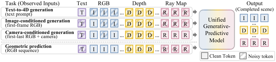
\[\mathcal{L} = \mathbb{E}_{t,\epsilon}\!\left[\sum_j a_j \lambda_{m(j)} \big\lVert \hat{v}_j - v_j^\star \big\rVert_2^2\right],\]

where $a_j \in {0,1}$ is the availability mask (1 if token $j$ has ground-truth supervision in this sample) and $\lambda_{m(j)}$ balances the four streams (RGB, depth, ray direction, ray moment). Five conditioning patterns are sampled during training, restricted by what each dataset annotates:

First RGB frame → rest of RGB + depth + rays (scene completion)
All RGB → depth + rays (RGB-to-geometry)
First+last RGB + all rays → middle RGB + depth (camera-controlled interpolation)
First RGB + all rays → rest of RGB + depth (camera-controlled extrapolation)
First RGB + all depth → rest of RGB + rays (depth-conditioned generation)

Imperfect history during training. Context tokens are not always forced to be perfectly clean: with probability $0.5$ they are clamped at $t_j=0$, and otherwise they receive a random lower noise level. Target tokens receive independently sampled higher noise levels. This teaches the model to use both perfectly clean context and imperfect context, which improves robustness at inference time when conditioning on generated or partially corrupted history.

3.4 Heterogeneous training

This is where the formulation pays off. Each training sample is represented in a common (RGB, depth, ray-map) format with a modality-availability mask; missing streams are filled with Gaussian placeholders, forced to maximum noise, and zeroed out of the loss. An RGB-only video clip and a fully annotated synthetic clip train the same model side by side; the loss simply lights up different terms. The per-modality losses are equally weighted, $\mathcal{L} = \tfrac{1}{4}(\mathcal{L}_I + \mathcal{L}_{R_d} + \mathcal{L}_{R_m} + \mathcal{L}_D)$, with availability masking applied within each term.

We train on a heterogeneous mixture of eight real, synthetic, and robotic video datasets that together cover different subsets of RGB, depth, camera pose, and text supervision (Table 1). Depth and pose for DL3DV-10K and ScanNet++ are obtained via the VIPE annotation pipeline . Captions are native for SpatialVID and AgiBot World; we additionally annotate DL3DV-10K and RealEstate10K with scene-level description prompts; the remaining datasets train without text conditioning. 7-Scenes is held out for evaluation only.

Table 1 · Training datasets and modality availability. ✓ = supervised; – = not used; (VIPE) = annotated via the VIPE pipeline; native = captions provided by the dataset; scene prompt = scene-level descriptions we annotated.

Dataset	Type	RGB	Depth	Camera pose	Text
RealEstate10K	real	✓	--	✓	scene prompt
DL3DV-10K	real	✓	✓ (VIPE)	✓ (VIPE)	scene prompt
SpatialVID	real	✓	--	✓	native
ScanNet++	real	✓	✓ (VIPE)	✓ (VIPE)	--
AgiBot World	robotic	✓	--	--	native
OmniWorld	synthetic	✓	✓	✓	--
Virtual KITTI 2	synthetic	✓	✓	✓	--
PointOdyssey	synthetic	✓	✓	✓	--
7-Scenes	eval-only	✓	✓	✓	--

3.5 Inference and test-time search

At inference, observed tokens are clamped to their clean values at every denoising step and assigned $t_j=0$; unknown tokens are denoised from Gaussian noise with UniPC (40 steps). A 50-frame clip takes $\sim$1 minute on one H100.

We additionally use history guidance , which is classifier-free guidance applied to the observed context rather than the text prompt:

\[\hat{v}_{\mathrm{HG}} = \hat{v}_{\mathcal{H}} + w_{\mathrm{hist}}\big(\hat{v}_{\mathcal{H}} - \hat{v}_{\varnothing}\big), \quad w_{\mathrm{hist}} = 2.0,\]

where $\hat{v}_{\mathcal{H}}$ has history clamped and $\hat{v}_{\varnothing}$ replaces it with noise.

Test-time search (TTS). Because the model defines a distribution over 4D scene completions, we can draw $L$ samples from different seeds with the same clamped context, giving $L$ joint hypotheses $\hat{S}^{(\ell)} = {(\hat{I}_i^{(\ell)}, \hat{D}_i^{(\ell)}, \hat{C}_i^{(\ell)})}$. We then score each candidate by cross-frame photometric reprojection using its own predicted depth and camera geometry:

\[e^{(\ell)} = \frac{1}{|\mathcal{P}|}\!\!\sum_{(i,j)\in\mathcal{P}}\!\!\frac{\big\lVert M_{ij}^{(\ell)} \odot (\tilde{I}_{i\to j}^{(\ell)} - \hat{I}_j^{(\ell)}) \big\rVert_1}{\lVert M_{ij}^{(\ell)} \rVert_1 + \epsilon},\]

with $\tilde{I}_{i\to j}^{(\ell)}$ the warp from frame $i$ to frame $j$, $M_{ij}^{(\ell)}$ the valid-pixel mask, and $\mathcal{P}$ an exhaustive pair set over a small anchor subsample. We pick $\ell^\star = \arg\min_\ell e^{(\ell)}$. Candidates whose RGB, depth, and rays disagree under their own geometry warp badly and self-eliminate. $L=16$ throughout.

Implementation notes (architecture, training, optimization, inference)

Base · Wan2.1-T2V-1.3B; 30 layers, hidden 1536, FFN 8960, 12 heads; VAE stride $[4,8,8]$, patch $[1,2,2]$; ray latents bypass the VAE and pack four consecutive 3-channel ray frames into a 16-channel latent.
Training · Conditioning patterns 1--5 in Sec. 3.3 are sampled per batch, restricted to each dataset's available modalities. Missing modalities use Gaussian placeholders forced to the maximum noise level and are masked out of the loss.
Optimization · AdamW, lr $1\!\times\!10^{-5}$, $(\beta_1,\beta_2)=(0.9,0.95)$, weight decay $0.05$, grad clip $5.0$, $1$k warmup, constant schedule; bf16 mixed precision; $4\times$ H200 GPUs, effective batch $16$ via grad-accum $4$, $\sim$$30$k steps; gradient checkpointing.
Inference · UniPC sampler with $40$ denoising steps and history-guidance strength $w_{\mathrm{hist}}=2.0$. A 50-frame clip at $240\times320$ takes approximately one minute on a single H100. TTS uses $L=16$ candidates and an anchor-pair photometric reprojection scorer.

4 · Experiments

We evaluate three tasks (camera-controlled generation, pose, depth) under dense (full RGB observed) and sparse (first+last RGB only) regimes, plus TTS on top of dense + sparse pose/depth. Baselines were chosen to test the unification claim against task-specialists.

4.1 Camera-controlled generation

Setup. First + last RGB + target camera trajectory are clamped; the model generates intermediate RGB. We evaluate PSNR/SSIM/LPIPS on RealEstate10K , DL3DV-10K , the 55-scene DL3DV-Evaluation split, and SpatialVID.

Baselines. Wan2.1-FLF-14B (no camera input) , a 14B-parameter first-last-frame video generator, roughly $10\times$ larger than our 1.3B model; DFoT , a diffusion-forcing video completer evaluated with camera conditioning; SEVA , a state-of-the-art NVS-specialist diffusion model.

Figure 4 · Camera-controlled generation. The first/last frames and a target camera trajectory (left) are clamped; each column on the right shows a candidate completion. Ours preserves dynamic content along the requested trajectory; SEVA is biased toward static scenes; Wan2.1-FLF has no camera input and drifts on complex motion; DFoT is camera-conditioned but can distort or remove moving humans. Use the dataset tabs and prev/next buttons to browse samples.

Table 2 · Camera-controlled generation. PSNR↑ / LPIPS↓ / SSIM↑. Best in bold blue, second in light blue.

Method	RealEstate10K			DL3DV-10K			DL3DV-Eval			SpatialVID
Method	PSNR	LPIPS	SSIM	PSNR	LPIPS	SSIM	PSNR	LPIPS	SSIM	PSNR	LPIPS	SSIM
Wan2.1-FLF	15.87	0.327	0.478	12.41	0.493	0.241	12.17	0.493	0.232	12.43	0.529	0.295
DFoT	21.23	0.178	0.680	14.15	0.438	0.368	14.33	0.365	0.328	14.71	0.408	0.389
SEVA	22.77	0.164	0.777	18.27	0.310	0.615	17.90	0.298	0.560	16.72	0.348	0.587
Ours	19.98	0.154	0.658	15.09	0.316	0.408	13.69	0.325	0.308	14.51	0.335	0.386

Analysis. We achieve the best LPIPS on RealEstate10K and SpatialVID and second-best on DL3DV, and we outperform Wan2.1-FLF on every metric on every dataset despite using roughly $10\times$ fewer parameters. SEVA wins on the pixel-aligned PSNR/SSIM; expected, since it is purpose-built for NVS. The interpretation: ray-map conditioning gives effective trajectory control under the same backbone that also predicts depth and pose; a specialist still beats us on pixel metrics, but we are competitive without specializing.

4.2 Camera pose estimation

Setup. RGB clamped; rays denoised; predicted ray maps are converted back to $(K, T)$. Dense: full video. Sparse: first+last frame only. Metrics: ATE, RPE$_t$, RPE$_r$ after Sim(3) Umeyama alignment, following Geo4D. Baselines: Geo4D , RayDiffusion .

Figure 5 · Predicted camera trajectories. Frustum wireframes for ground truth, our model, Geo4D, and RayDiffusion. Use the dataset tabs and prev/next buttons to browse samples.

Table 3 · Pose estimation. ATE↓ / RPE$_t$↓ / RPE$_r$↓ ($\times!10^{-2}$).

	Method	RealEstate10K			DL3DV-10K			ScanNet++			SpatialVID
		ATE	RPE$_t$	RPE$_r$	ATE	RPE$_t$	RPE$_r$	ATE	RPE$_t$	RPE$_r$	ATE	RPE$_t$	RPE$_r$
Dense	RayDiffusion	5.712	7.216	11.560	5.840	9.569	35.970	2.824	4.082	53.920	6.262	8.610	31.840
	Geo4D	1.103	0.559	0.232	1.868	0.625	0.911	1.716	0.472	0.937	2.533	0.767	0.577
	Ours	0.593	0.222	0.952	1.160	0.351	2.300	1.169	0.337	2.372	2.117	0.702	1.581
	Ours (TTS)	0.534	0.220	0.966	1.208	0.356	2.381	0.927	0.323	2.316	2.169	0.701	1.464
Sparse	RayDiffusion	13.715	24.220	48.851	10.185	22.503	77.655	4.475	14.263	109.84	14.486	33.801	86.099
	Geo4D	26.516	37.499	14.980	16.156	22.848	55.886	8.875	12.551	71.614	30.888	43.682	45.924
	Ours	1.220	0.326	0.984	2.261	0.589	2.938	2.229	0.518	3.602	3.683	0.992	2.055
	Ours (TTS)	1.088	0.319	0.951	2.398	0.611	3.123	2.031	0.518	3.270	3.762	1.021	2.202

Analysis. Dense: we beat both baselines on ATE / RPE$_t$ on every dataset, e.g. DL3DV ATE 1.868 → 1.160 (38% lower) vs Geo4D. Geo4D wins on rotation RPE$_r$ where its specialized geometry head helps, but we gain on global trajectory. Sparse: the order-of-magnitude gap is the most informative number on this page. With only two RGB frames, both RayDiffusion and Geo4D collapse (ATE 10–30); we stay at 1–4 by falling back on the joint RGB+camera prior learned from heterogeneous data. SpatialVID sparse ATE 30.888 → 3.683 — the kind of regime where a feedforward predictor has nothing to match locally and a generative posterior is genuinely the right tool.

4.3 Depth prediction

Setup. RGB clamped; depth denoised. Evaluation on Virtual KITTI 2 , DL3DV-10K, ScanNet++ , and 7-Scenes ; video-level scale-and-shift alignment, then Abs Rel, RMSE, $\delta!<!1.25$. Baselines: Geo4D, ChronoDepth .

Figure 6 · Video depth qualitative. RGB · GT depth · ours · Geo4D · ChronoDepth. Use the dataset tabs and prev/next buttons to browse samples; ours preserves sharper object boundaries and more coherent temporal structure.

Table 4 · Depth prediction. AbsRel↓ / RMSE↓ / $\delta!<!1.25$↑.

	Method	Virtual KITTI 2			DL3DV-10K			ScanNet++			7-Scenes
		Rel	RMSE	$\delta$	Rel	RMSE	$\delta$	Rel	RMSE	$\delta$	Rel	RMSE	$\delta$
Dense	ChronoDepth	0.382	0.287	0.399	0.340	0.161	0.509	0.185	0.208	0.796	1.443	0.294	0.381
	Geo4D	0.211	0.194	0.675	0.304	0.206	0.631	0.150	0.191	0.863	1.362	0.258	0.531
	Ours	0.225	0.189	0.680	0.308	0.171	0.545	0.297	0.201	0.749	1.387	0.260	0.607
	Ours (TTS)	0.220	0.183	0.695	0.304	0.175	0.570	0.251	0.218	0.736	1.385	0.259	0.619
Sparse	ChronoDepth	1.309	0.412	0.127	0.835	0.284	0.274	0.689	0.292	0.500	1.431	0.268	0.483
	Geo4D	1.309	0.412	0.127	0.855	0.288	0.268	0.699	0.296	0.486	1.371	0.223	0.737
	Ours	0.747	0.632	0.401	0.731	0.369	0.422	0.418	0.272	0.655	1.451	0.274	0.486
	Ours (TTS)	0.716	0.573	0.449	0.670	0.291	0.397	0.454	0.280	0.695	1.445	0.272	0.498

Analysis. Dense: we are competitive everywhere and lead on Virtual KITTI 2 RMSE and 7-Scenes $\delta$. Geo4D remains stronger on the indoor ScanNet++ split; specialist geometry models still benefit from indoor-heavy training. Sparse: the joint formulation wins decisively on Virtual KITTI 2, DL3DV, and ScanNet++ (AbsRel 0.689 → 0.418 on ScanNet++). Two frames are not enough for video-depth-specialists to exploit temporal context; the generative prior plus cross-modal training is.

4.4 Test-time search

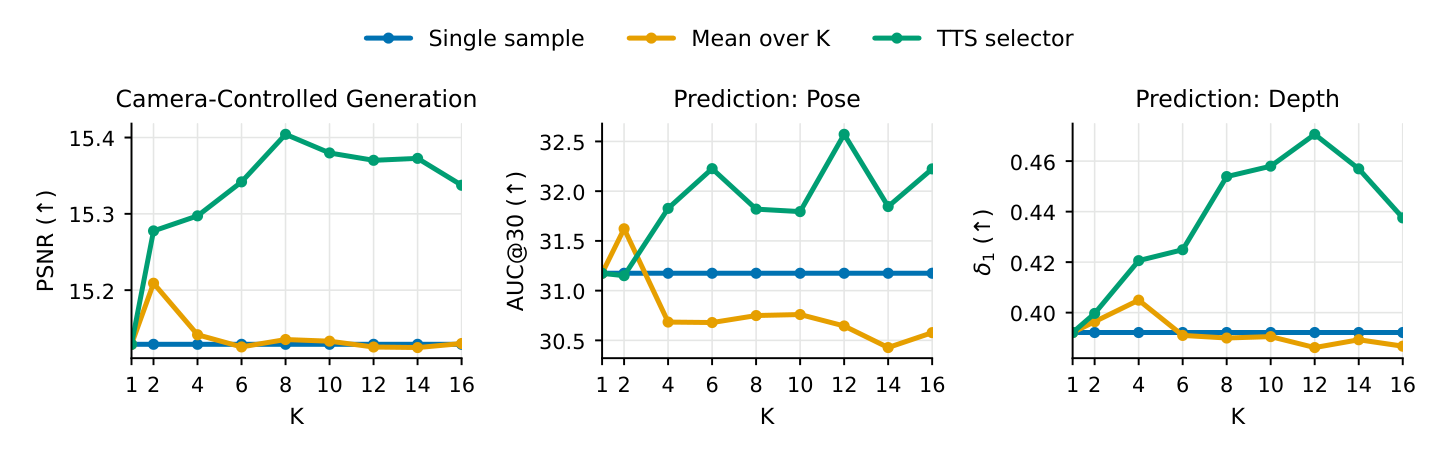
TTS curves. — **Figure 7 · Test-time search** on DL3DV-10K. Pose ATE and depth AbsRel improve as we sample more candidates and pick the one with the lowest RGB reprojection error. No retraining, no extra parameters: just more inference compute spent in the right place.

The TTS rows in Tables 3 and 4 are the same model, with $L=16$ samples and reprojection-based selection. TTS improves on the no-search baseline in 9/12 pose cells (dense) and 11/12 depth cells (sparse). Gains are not uniform: reprojection error is a proxy for geometric accuracy, so on textureless or specular regions the selector is misled. Still — improvements at zero training cost, monotone in $L$ on DL3DV (Fig. 7), and consistent with the cognitive view of perception as generate-and-check .

5 · Discussion, limitations, and outlook

The headline finding is that one model + one mask is enough. A 1.3B-parameter diffusion transformer with three modality streams and shared attention, trained with diffusion forcing on heterogeneous data, handles camera-controlled generation, video depth, and camera pose, and improves itself at inference time by sampling more 4D scene hypotheses. The conditional-completion formulation cleanly answers our scientific question: generation and prediction are the same problem, and the benefits (heterogeneous supervision, joint priors, posterior search) are concretely measurable, especially in sparse regimes.

Implications. (i) Web-scale RGB-only video can train geometry models without needing matched depth or pose. (ii) Sparse-view geometry (a regime where feedforward predictors collapse) becomes the strength of generative scene models, not a weakness. (iii) Inference compute is a usable lever for accuracy.

Limitations. (1) Specialist NVS models like SEVA still win on pixel-aligned PSNR/SSIM; spending capacity on geometry costs some appearance fidelity. (2) The TTS scorer is photometric reprojection, which fails on low-texture or specular surfaces; a learned multimodal consistency score would likely improve search. (3) We train at $240\times320$, 50 frames, on 4 H200s — modest resolution and scale by current video-model standards. (4) Indoor depth still favors specialist geometry models; a better dataset balance would close that gap.

Looking ahead. Stronger learned consistency scorers, search during the denoising process (not just over seeds), larger-scale training, and embodied/robotic evaluation are the natural next moves. The structural point survives: stop thinking of “generation” and “prediction” as separate capabilities. They are different conditional queries on the same joint distribution, and a diffusion transformer can learn that distribution from messy, partially annotated video at scale.