one model, four dimensions: generating and predicting scenes together

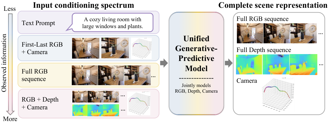
RGB video, depth, and camera pose are three views of the same 4D scene. Treating them as missing-modality completion in a single diffusion model means generation and prediction stop being separate problems.

The setup

A single image, or even a short video clip, only ever shows you part of a scene. If you want a model to understand what it is looking at, “understanding” has to include things the camera didn’t capture: the unseen sides of objects, where the camera was, how far away each surface is, and how all of that will evolve a few seconds later.

The field has, until now, mostly split that job in two. Feedforward predictors estimate depth, pose, and 3D structure directly from pixels — fast, often accurate, but they give you one deterministic answer that gets brittle when observations are sparse. Generative video models hallucinate beautifully but have no idea what a meter is. Bolting them together pipeline-style works only when one stage is willing to accept the other’s output as gospel, and that is rarely a good assumption.

The point of this project is small and stubborn: generation and prediction are the same problem. Both are conditional completion of a partially observed 4D scene. The only thing that changes between “make a video from a text prompt” and “estimate camera pose from a video” is which tokens you happen to be holding fixed.

One model, many queries. Given any partial observation --- a text prompt, a single image, an RGB sequence, camera poses, or a depth map --- the same model fills in the rest. Camera-controlled generation, depth estimation, and pose recovery all fall out of the same denoising objective.

One representation for appearance and geometry

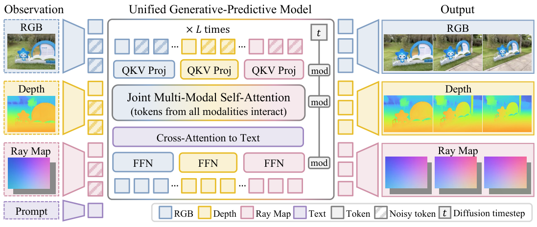
A frame of the world, in this model, has three spatially aligned channels:

• RGB $I_i$ — appearance.
• Depth $D_i$ — visible 3D structure.
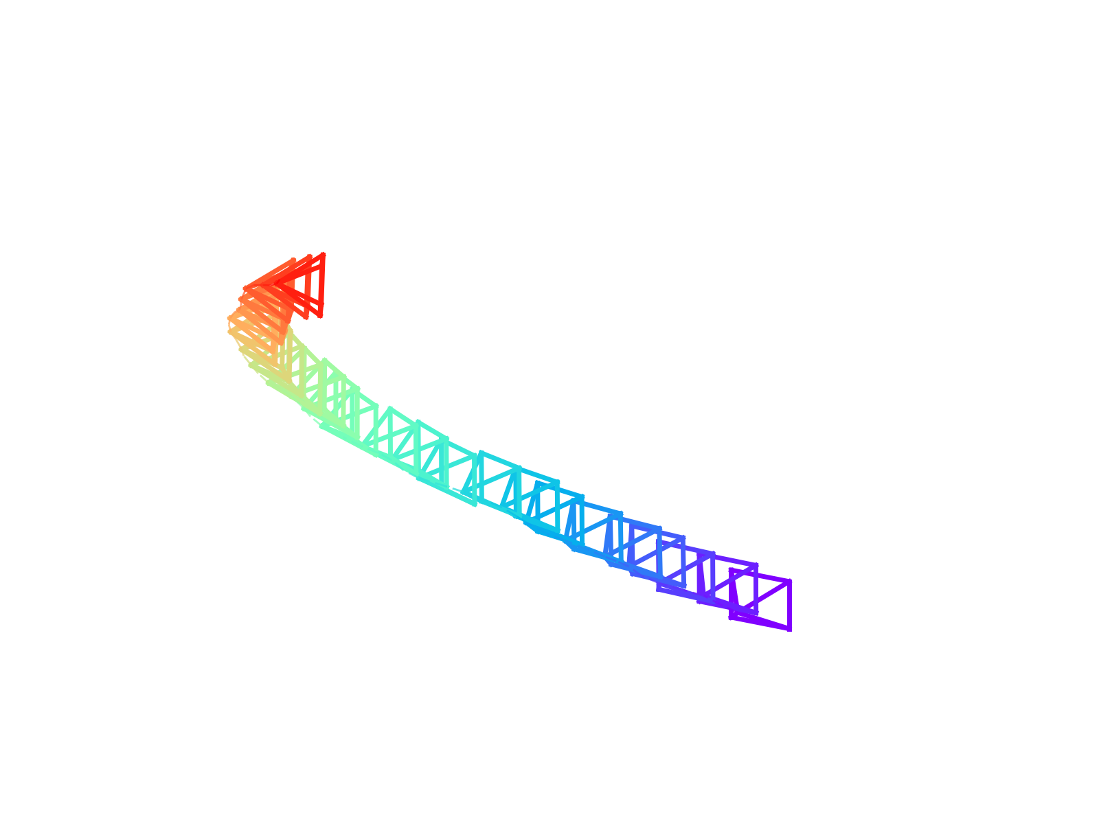
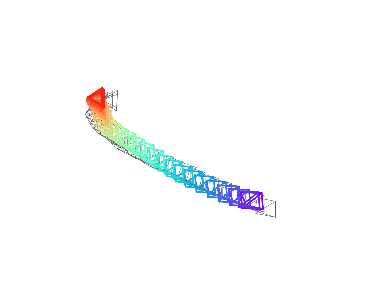
• Camera rays $R_i$ — viewpoint, written as a dense ray map with a ray direction $\mathbf{d}_i(u,v)$ and a Plücker moment $\mathbf{m}_i(u,v) = \mathbf{o}_i \times \mathbf{d}_i(u,v)$ at every pixel.

Why bother turning camera pose into an image? Because once it is image-shaped, you can token-ize it the same way you token-ize RGB and depth, and a transformer can mix the three through ordinary self-attention. No bespoke camera encoder, no awkward cross-attention scheme — camera geometry just becomes another channel in the same latent grid.

A shared scale-and-shift normalization on depth and camera pose makes cross-modal constraints (like reprojection error) numerically well-defined, which matters later when we want to search over candidate scenes.

A single trick called diffusion forcing

Once everything is tokens in a shared sequence, training is one line of intuition: observed tokens get zero noise; missing tokens get full noise. A standard diffusion transformer denoises the noisy ones, conditioned on the clean ones.

Per-token noise levels turn one model into many. Clean = "you observed this." Noisy = "fill this in." The pattern decides the task.

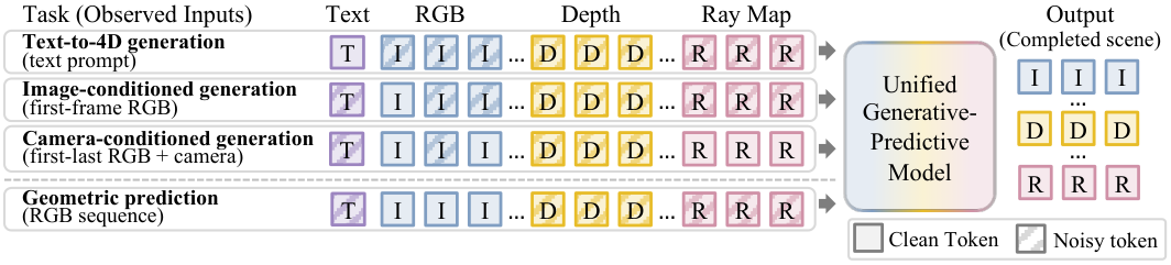
So one architecture covers all of these by choosing a different mask:

Mask pattern	Task
first RGB frame clean, rest noisy	text/image-to-video
first + last RGB + all rays clean	camera-controlled interpolation
all RGB clean, depth + rays noisy	depth + pose estimation
all depth clean, RGB + rays noisy	depth-conditioned generation

The model never sees a “task label.” It sees noise levels.

The architecture. RGB and depth go through a VAE encoder; ray maps are projected directly; everything is processed by a shared multimodal transformer with modality-specific projections and spatiotemporal RoPE. Output tokens decode back to RGB, depth, and dense ray maps, which convert to camera parameters.

What you get for free

Two practical consequences fall out of the formulation, and they are the parts I actually find surprising:

Heterogeneous data. The web has billions of videos with no depth or pose, plenty with pose only, and a much smaller pile with both. Most pipelines have to throw away examples that don't have every modality. Diffusion forcing doesn't.

1. Arbitrary conditioning at inference. Hand the model whatever you have at test time — a prompt, a frame, a frame plus camera intrinsics, a sequence plus depth — and ask for whatever you want. Same weights.

2. Heterogeneous supervision at training. The loss only applies to available target modalities. So an RGB-only YouTube clip and an RGB+depth+pose synthetic clip can train the same model side by side. No alignment surgery, no separate heads.

Does it work?

The model is a 1.3B-parameter diffusion transformer initialized from Wan2.1-T2V, fine-tuned on a mixture of DL3DV-10K, RealEstate10K, ScanNet++, SpatialVID, AgiBot World, and a few synthetic sets. 50-frame clips at 240×320, 10 fps, four H200s.

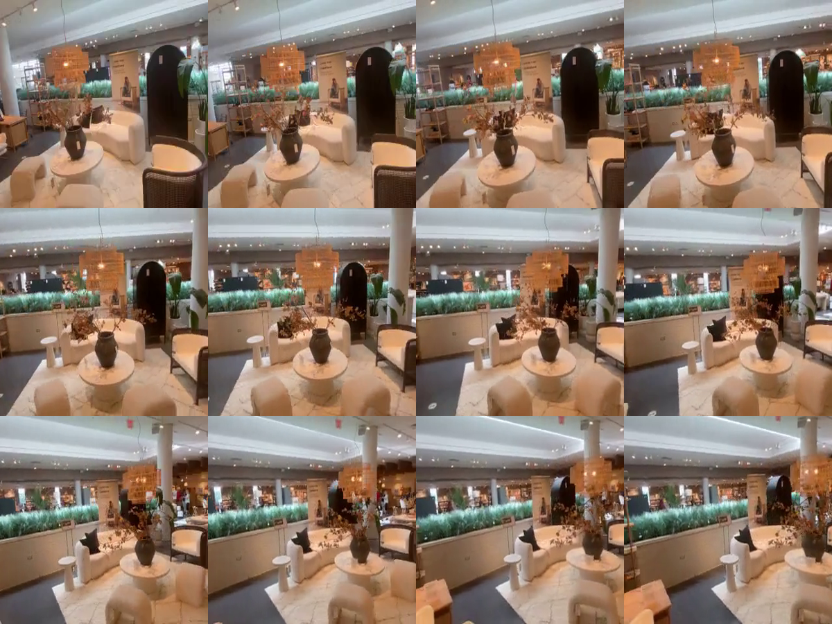
Camera-conditioned generation

Given the first and last frame plus a target camera trajectory, the model fills in the intermediate video. It’s competitive with specialized novel-view-synthesis systems on perceptual quality (best or second-best LPIPS across RealEstate10K, SpatialVID, DL3DV, DL3DV-Eval), and noticeably better than first-/last-frame generative baselines like Wan2.1-FLF or DFoT at staying on the requested trajectory. SEVA, a task-specific NVS model, still wins on pixel-aligned PSNR/SSIM — the tradeoff for spending capacity on appearance and geometry.

Camera pose from video

Predict the ray map, convert to camera parameters, compare against ground truth. In the dense setting (full video observed), our model improves ATE and translation RPE on all four evaluation datasets over both Geo4D and RayDiffusion.

input video (DL3DV)

ground truth

ours

Headline number.
ATE on DL3DV-10K:
Geo4D → 1.868
Ours → 1.160

~38% lower trajectory error, same model that also does generation.

The sparse setting is the more interesting one. With only the first and last frames, local feature matching can’t help you — the model has to fall back on a learned prior over plausible trajectories between two views. It still produces reasonable cameras, which I read as evidence that the joint RGB+pose training has actually learned a world prior and not just a fancy SfM front-end.

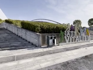
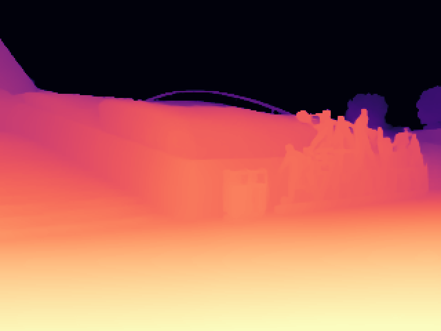
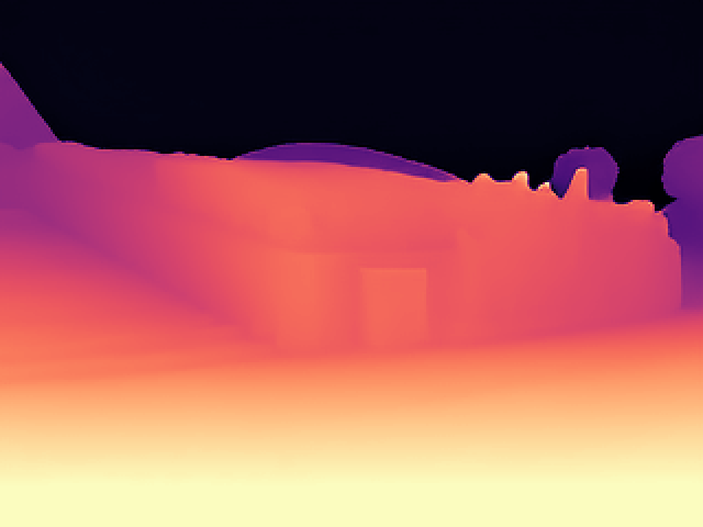
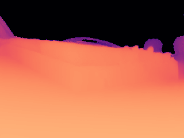
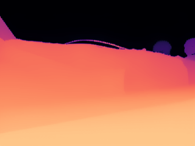
Video depth

Same model, different mask: RGB clean, depth noisy. Across Virtual KITTI2, DL3DV-10K, ScanNet++, and 7-Scenes the model is competitive with specialized video depth methods like ChronoDepth and Geo4D, with the best $\delta < 1.25$ on 7-Scenes. In the sparse two-image regime it outperforms both on several metrics.

RGB · GT · ours · Geo4D · ChronoDepth (DL3DV sample).

Search at inference time

Here’s a thing you can do with a generative model that you can’t do with a feedforward predictor: draw several samples, score them, keep the best. Because RGB, depth, and rays are sampled jointly, you can score a sample by re-projecting it through its own predicted geometry and measuring photometric consistency against the observations. That’s a cheap, parameter-free posterior approximation.

Pose and depth metrics improve monotonically with the number of candidate samples on DL3DV-10K. No retraining, no extra parameters --- just more inference compute spent in the right place.

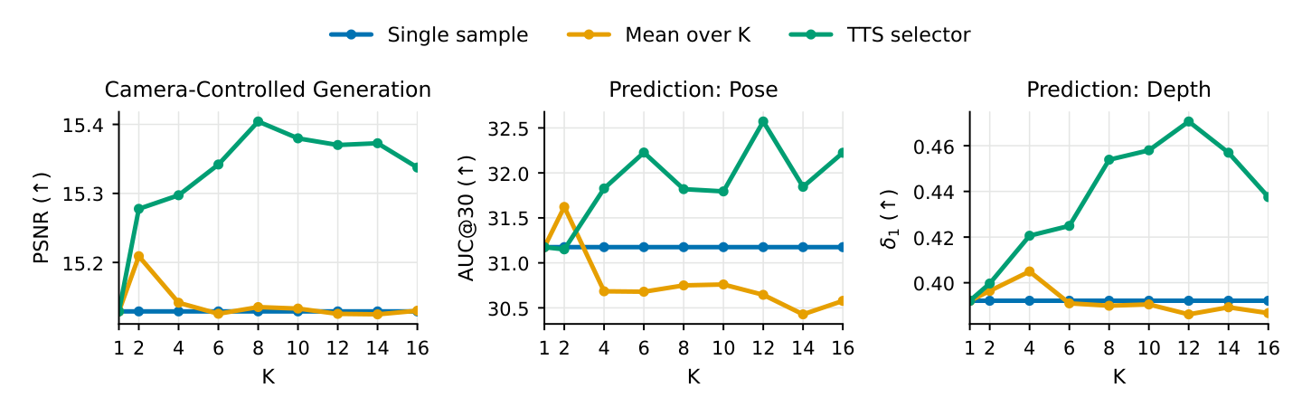
This is the part that I think is philosophically the most fun. Perception as inference — the idea that vision is generating-and-checking against an internal world model — has been in cognitive science forever. Diffusion plus a joint scene representation gives you the simplest possible computational instance of it: you literally generate scenes and pick the one whose geometry best explains the pixels.

Full appendix tables (PSNR/SSIM/LPIPS, AbsRel/RMSE/$\delta$, ATE/RPE per dataset and method)

Coming once the paper is on arXiv --- this post is the short version.

Where this is going

A few honest limitations: specialized novel-view models still beat us on pixel-aligned metrics; the test-time scorer is RGB reprojection, which fails on textureless or specular regions; and 240×320 is not yet the resolution at which video models impress people. None of these feel fundamental — they feel like dials to turn.

What does feel structural is the formulation: once you stop thinking of “generation” and “prediction” as different capabilities and start thinking of them as different conditional queries on the same joint distribution, a lot of design decisions get easier. There’s nothing left to choose between a video model and a perception model. There’s just one model and a noise mask.

---

If you want the technical version: the paper is on arXiv with full tables, the appendix, and training details. This post compresses ~9 pages of dense methods prose into the part I’d want to read first.